Introduction
I’ve been curious about how the places I spend my time affect my behavior. Am I more productive in the library or my dorm room? Do I run faster in my favorite park or at the gym?
To answer these questions I first need to classify the places I spend my time. To do that I chose to run a clustering algorithm.
During my undergraduate years at Michigan State University I frequented a lot of places on campus. Some of these areas were inside, some were not. Some were large parks and some were limited to a single lab. To categorize all these areas I want to use a clustering algorithm that can take into account both where I was and how much time I spent there. This is where DBSCAN comes into play.
DBSCAN
DBSCAN is density-based clustering algorithm. Density clustering works by classifying areas of high density separated by areas of low density. Through this method you don’t need to worry about the shape, size, or number of clusters, only how the data points are separated.
DBSCAN uses a few core concepts:
- Density = number of points within a specified radius Epsilon (Eps)
- A core point is a point that has more than the specified number of neighbors (MinPts) within Eps (including the point itself)
- A border point has fewer than MinPts within Eps, but is in the neighborhood of a core point
- A noise point is any point that is not a core point or a border point.
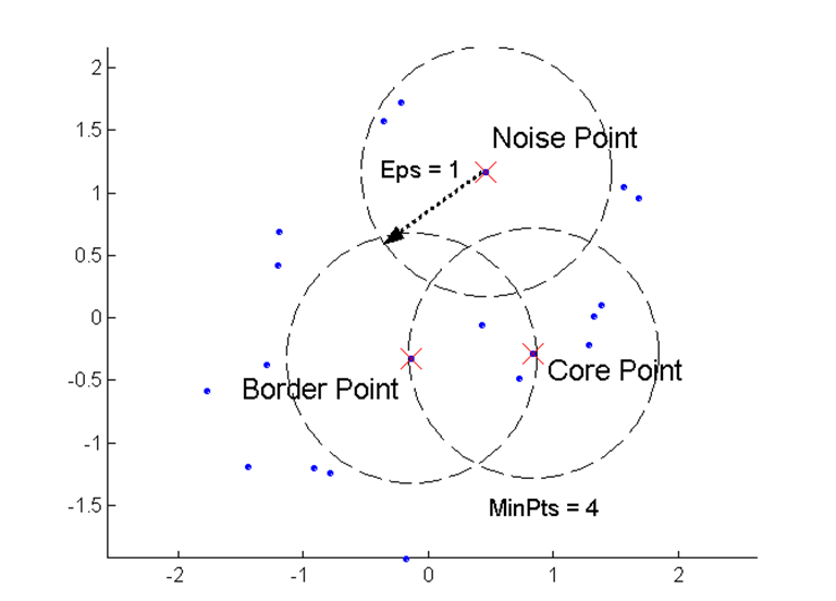
Illustration of DBSCAN points
With GPS location data, you can use DBSCAN to find clusters of places. Additionally, you can use the amount of time spent in a location to apply weight to a point. This way both time and distance contribute to forming clusters.
Google Location History
If you use an Android phone and haven’t turned off location tracking, then you likely have many days, months, or years of location history stored by Google. You can download this history using Google Takeout. This is the same data that Google uses to make their timelines.
Import the Data
To import your Google location history go to Google Takeout, toggle “Location History”, and create the archive. You will get a JSON file of all the locations Google has tracked. Put this in an easy-to-use location. You will also see some metadata such as Google’s best guess at how fast you were moving and what activity you were doing.
Formatting JSON History
There is some formatting that will have to be done to get the JSON file into a tidy R dataframe.
The file can be rather large. If it is too large for your computer to read using fromJSON, you can try to convert to NDJSON and stream it. I’d recommend first trying to manage memory by removing what you don’t need with rm() and gc().
The first thing I always load up in R is Tidyverse. Because why would you not want to use it.
library(tidyverse)Get your data with jsonlite
library(jsonlite)

file_name <- "../data/Location History.json"

system.time(json.data <- fromJSON("../data/Location History.json"))
All the data is nested under a JSON object called locations. fromJSON will return a list, which you can use to grab the object.
json.location <- json.data$locationsFormat latitude, longitude, and time to standard formats.
json.location$time <- as.POSIXct(as.numeric(json.location$timestampMs)/1000, origin = "1970-01-01")
# converting longitude and latitude from E7 to GPS coordinates
json.location$lat = json.location$latitudeE7 / 1e7
json.location$lon = json.location$longitudeE7 / 1e7
Save data into an RDS, where it will be faster to load in the future.
saveRDS(json.location, "../data/location_history.rds")loc <- readRDS("../data/location_history.rds")Later, when running DBSCAN, you will likely be limited by the amount of memory your computer has available. Here are some pointers to limit the amount of memory needed.
- Filter to the area you’re interested in
- Group on an approximate location
- Remove obvious noise points
First, I’m going to filter out any locations tracked outside of MSU and round all my latitude and longitude points to approximate exact locations.
filtered.loc <- loc %>%
  select(-activity, -latitudeE7, -longitudeE7) %>%
  filter(time > as.Date("2014-08-28"), time < as.Date("2018-05-15"),
         lat > 42.72, lat <42.74, lon > -84.495,  lon < -84.47 ) %>%
  mutate(lat = round(lat, 4), lon = round(lon, 4))
Now, to make the dataframe as small as possible I group on the approximate location and sum the amount of time at each point.
When aggregating the time spent in one location you will need to deal with gaps in the GPS data. I’m creating a maximum time spent in one place without an update. This way, if I lost GPS connection for 2 hours it will only count as 10 minutes in the last location seen.You may want to use a different approach to clean errors in the GPS data.
You could incorporate a change in location to determine if the GPS didn’t update over a long period and adjust or throw out that data. Cleaning this data could be an interesting machine learning project in itself. You can even see some manual cleaning techniques in Google’s Timeline Interface, such as asking users to confirm locations.
#max.difference is in minutes
max.difference = 10
time.per.loc <- filtered.loc %>%
  arrange(desc(time)) %>%
  mutate(raw.diff = as.numeric(time - lead(time), units = "mins"),
         diff = case_when(
           raw.diff >= max.difference ~ max.difference,
           raw.diff < max.difference ~ raw.diff,
           TRUE ~ 0)) %>%
  group_by(lon, lat) %>%
  summarise(total_time = sum(diff, na.rm = TRUE)) %>%
  ungroup() %>%
  filter(!is.na(total_time))
Now check what the data looks like. This will be the basic format to run DBSCAN on. I have 10840 rows, which runs well on my 8GB of data. If yours is large, you may need to attempt more methods at decreasing the amount of points you need to analyze.
nrow(time.per.loc)## [1] 10840summary(time.per.loc)## lon lat total_time
## Min. :-84.50 Min. :42.72 Min. : 0.01
## 1st Qu.:-84.49 1st Qu.:42.72 1st Qu.: 1.03
## Median :-84.48 Median :42.73 Median : 2.93
## Mean :-84.48 Mean :42.73 Mean : 55.56
## 3rd Qu.:-84.48 3rd Qu.:42.73 3rd Qu.: 10.18
## Max. :-84.47 Max. :42.74 Max. :97855.86View Location
Due to new updates with Google’s map API, there are a few new changes you need to make to use Google Maps for plotting. Essentially, you need to make sure you have an API key and register it in your R session.
Roman Abashin goes through the steps in a helpful tutorial here.
google.api.key <- "your.api.key"library(ggmap)register_google(key=google.api.key)
msu <- get_googlemap(center = c(lon = -84.48178, lat = 42.72816), zoom = 15) I recommend saving the map to avoid unnecessary repeat calls to Google’s map API. Also, it helps for working offline.
save(msu, file = "../data/msu_map.RData")load(file = "../data/msu_map.RData")Now I can see all the time I spent on campus.
ggmap(msu) + geom_point(data = time.per.loc, aes(x = lon, y =lat, color = total_time, alpha = total_time, size = total_time)) 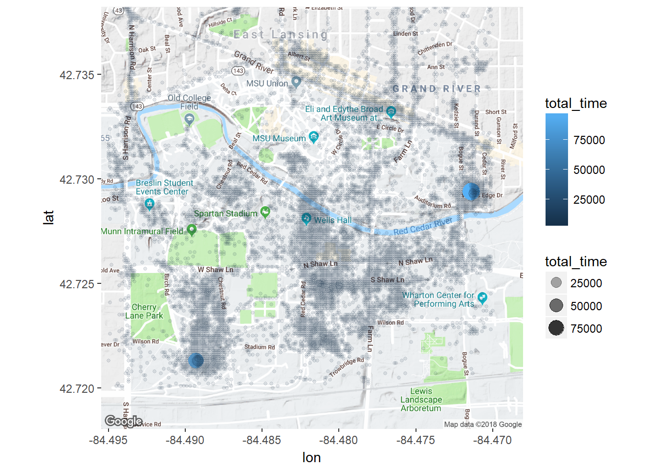
Even before using clustering, I can see a couple spots that stand out as single lat,lon positions where a lot of time was spent. Down in the south west was my dorm room freshman year and over in the east was my girlfriend’s apartment.
However, it’s hard to assign much meaning to all the other places. Time to employ some clustering.
Running DBSCAN
There are two parameters to set when using DBSCAN - minPts and eps. With the weight of time, minPts becomes the minimum amount of time spent in a potential cluster. With a fixed minPts, we can determine eps through a nearest neighbor graph.
Within a cluster, each point’s distance to the kth nearest neighbor will be roughly the same, but noise points will be farther away.
library(spatstat)
distances <- nndist(time.per.loc$lon, time.per.loc$lat, k = 5)
plot(sort(distances), main = "Distances to 5th Neighbor", xlab = "Sorted Points", ylab = "Distance")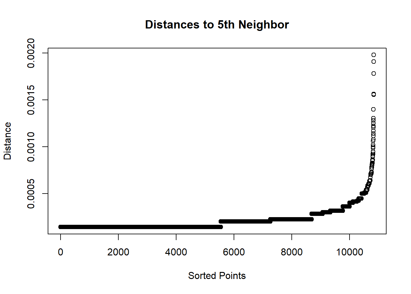
From here we can pick the inflection point for how far minEps should be. It looks like somewhere between 0.0000 and 0.0005.
However, when using time as a weight, minPts is no longer a representation of a number of neighbors. Rather, minPts is measured in minutes. To do the same analysis with weighted minutes, there is some manipulation we can do.
View Time Spent Over Distances.
First, get the distances to some k neighbors. Using the get.knn function from the FNN library we can easily retrieve the index of a neighbor point. This will be necessary for mapping a point back to how much time was spent there.
library(FNN)
max.neighbors <- 100
location.matrix <- matrix(c(time.per.loc$lon, time.per.loc$lat), ncol=2)
knn.vals <- get.knn(location.matrix, k=max.neighbors, algo="kd_tree")
There are a lot of outliers where I spent a large amount of time in an exact location, such as my dorm room. To deal with these points I’m setting a maximum amount of time to allow one position.
#set time (equivalent to k for normal dbscan)
min.time <-  60 * 10
#for outliers
adjusted_times <- time.per.loc$total_time
# cutoff <- sd(time.per.loc$total_time) * 3
cutoff <- min.time - 1
adjusted_times[adjusted_times > cutoff] <- cutoff
This function maps each index to the time spent at that point. The weighted distance will show how much time was spent in each neighbor point.
weighted.distances <- knn.vals$nn.index
weighted.distances[] <- vapply(knn.vals$nn.index,function(x)adjusted_times[x], numeric(1))
To get how much time was spent within a region we need to sum up the time for all points up to the kth neighbor. To do this, I loop through each column and take the dot product of all previous columns with a vector of ones.
summed.distances <- weighted.distances
for(k in 2:max.neighbors){
  summed.distances[,k] = weighted.distances[,1:k] %*% rep(1, k)
}
With summed.distances we have how much time it takes to get to kth neighbor. Now we can use the distances we have from get.knn and find the distance it takes to get to an amount of time.
#map matrix to 1 if above time at nth neighbor, 0 if below
above.time.matrix <- summed.distances >= min.time
above.time.matrix[] <- vapply(above.time.matrix, as.numeric, as.numeric(1))

#multiply distance matrix to get either the distance or 0 if not at min time
distance.matrix <- knn.vals$nn.dist * above.time.matrix
#convert 0 to NA so we can use min function to find smalles
distance.matrix[distance.matrix == 0] <- NA
min.distances <- apply(distance.matrix, 1, min, na.rm = TRUE)
plot(sort(min.distances),
main=paste("Points sorted according to distance to accumulate",
min.time/60,
"hours"),
xlab = "Sorted Points", ylab = "Distance")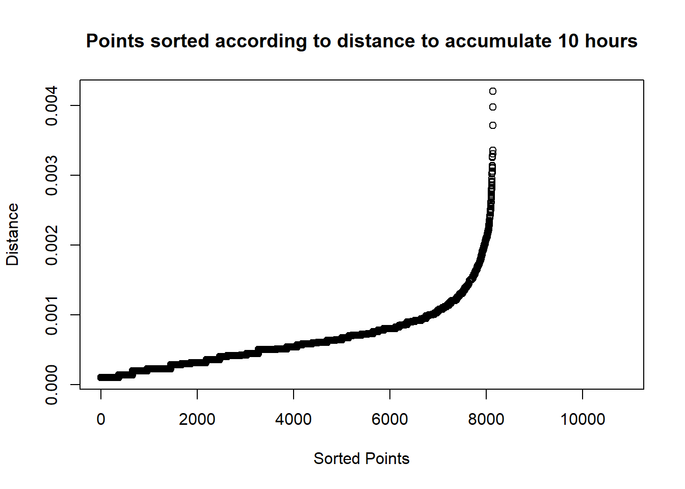
Finally, we have an idea of how the points are distributed in terms of time spent nearby. We can use this information to set a proper eps.
Run DBSCAN
There are two libraries that provide DBSCAN capability: FPC and dbscan. FPC has more functionality, but is slower. dbscan was written in C++ using k-d trees to be faster. dbscan has fewer capabilities, but since location will be using euclidean distance, it will work perfectly.
library(dbscan)
dbscan.time.per.loc <- time.per.loc
dbscan.time.per.loc$adjusted_time <- adjusted_times
db.loc <- dbscan(location.matrix, eps = 0.0004, minPts = min.time, weights = adjusted_times)
dbscan.time.per.loc$cluster <- db.loc$cluster
View the Results
Formatting Results
Cluster 0 is for noise points so I removed it. It also is helpful to change the cluster into a factor as it has no numeric value.
db.data <- dbscan.time.per.loc %>%
  filter(cluster != 0) %>%
  mutate(cluster = as.factor(cluster))
Generate Cluster Centers
cluster.centers <- db.data %>%
  group_by(cluster) %>%
  summarise(lon = round(mean(lon), 6), lat = round(mean(lat), 6), total_days = round(sum(total_time)/60))
You can also use reverse geocode to get text names for each cluster based on the center location.
cluster.centers$textAddress <- mapply(FUN = function(lon, lat) revgeocode(c(lon, lat))[[1]], cluster.centers$lon, cluster.centers$lat)Map Clusters
library(directlabels)
ggmap(msu) + geom_point(data = db.data, aes(x = lon, y =lat , color = cluster), alpha = .5) +
  geom_point(data=cluster.centers, aes(x = lon, y = lat),
             alpha = 1, fill = "black", pch = 21, size = 2) +
  geom_dl(data = cluster.centers, aes(label = total_days), method = list(dl.trans(y = y + 0.3),
                                                            cex = .8, fontface = "bold")) +
  theme(legend.position="none")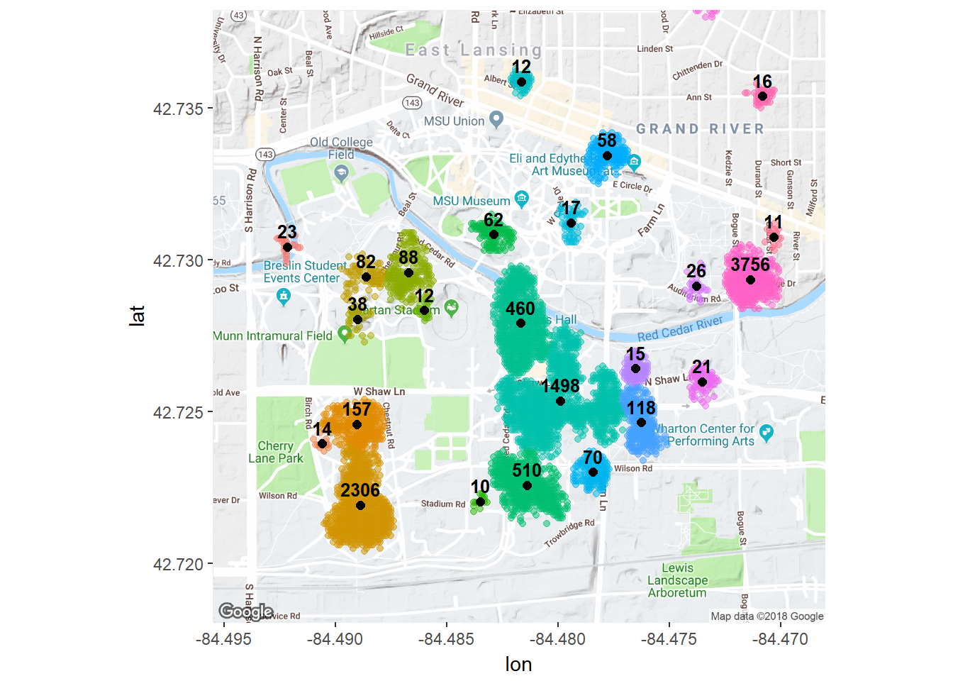
There we have it: places clustered by time and distance. These clusters can be paired with other data to analyze differences by location. I hope you enjoy running through this on your own location history.