Introduction
I love Spotify’s curated music. I can usually find something I want to listen to. Yet, even with my lists of favorites and my Discover Weekly playlist I still come across plenty of songs that I’m not feeling and have to skip. I found myself wondering what factors determine whether I skip a song or finish it, and set out to use my Spotify data to predict when I’m going to skip a song.
Include the Libraries
I’m going to be analyzing in R with the following packages.
library(tidyverse) # make R fun
library(randomForest) # create Random Forest ML Model
library(jsonlite) # parse spotify data
library(httr) # request data from spotify API
library(lubridate) # reformat dates
library(rlist) # manipulate spotify data
Getting the Data
You can download the last 90 days of your listening history through the Spotify website. Here’s a tutorial to help you find the menu to download. I’m not sure why they only provide 90 days, and unfortunately I don’t know any other way to get this data. You can try to use Scrobble with last.fm, but that won’t give you the duration you listened to a song.
Once you have downloaded your data, you can find your listening history in the StreamingHistory.json file.
streaming_history <- read_json("../data/StreamingHistory.json",
                             simplifyVector = TRUE,
flatten = TRUE)str(streaming_history)## 'data.frame': 3654 obs. of 4 variables:
## $ endTime : chr "2018-11-19 17:45" "2018-11-19 17:48" "2018-11-19 17:52" "2018-11-19 17:58" ...
## $ artistName: chr "Maribou State" "Will Stratton" "Elder Island" "Shanic" ...
## $ trackName : chr "Beginner's Luck" "Hemet Pine Singer" "Welcome State" "It All Changed So Fast" ...
## $ msPlayed : int 268027 191735 270476 342857 188664 182783 148155 163813 225973 226976 ...We can use the Spotify search API to retrieve the track ID and other feature data from Spotify. For the auth token, you can use the token generated within the API testing interface on Spotify’s document website. It expires fairly quickly, but nothing we’re doing here requires querying for too long.
auth_code = paste("Bearer", "[Your-Code-Here]")This function will search Spotify for a song and get the metadata that we’re interested in. Duration will be used to determine whether a song was skipped, popularity can be used as a feature, and additional IDs can be used to get more metadata for additional features.
get_track_metadata <- function(artist_name, track_name){
  #Search Tracks
  # track_name <- "4AM in London"
  # artist_name <- "Benjamin Francis Leftwich"
  search <- paste("track:", track_name, "artist:", artist_name)

  query_response <- GET("https://api.spotify.com/v1/search",
                        add_headers(Authorization = auth_code),
                        query = list(
                          q = search,
                          type = "track",
                          market="US"
                        )
  )
  #get the json response
  parsed_query_response <- content(query_response, "parsed")
  track_id <- tryCatch(parsed_query_response$tracks$items[[1]]$id,
                       error=function(e) NA)
  track_duration <- tryCatch(parsed_query_response$tracks$items[[1]]$duration_ms,
                             error=function(e) NA)
  track_popularity <- tryCatch(parsed_query_response$tracks$items[[1]]$popularity,
                               error=function(e) NA)
  track_album_id <- tryCatch(parsed_query_response$tracks$items[[1]]$album$id,
                             error=function(e) NA)
  track_artist_id <- tryCatch(parsed_query_response$tracks$items[[1]]$album$artists[[1]]$id,
                              error=function(e) NA)

  data.frame(track_id = track_id,
             track_album_id = track_album_id,
             track_artist_id = track_artist_id,
             track_duration = track_duration,
             track_popularity = track_popularity
  )
}
Loop through every record and get the track metadata.
track_metadata <- data.frame(track_id = c(),?

       track_album_id = c(),
       track_artist_id = c(),
       track_duration = c(),
       track_popularity = c()
  )
#nrow(streaming_history)
for (row in 1:nrow(streaming_history)) {
  # print(streaming_history[row,])
  track_name <- streaming_history[row,]$trackName
  artist_name  <- streaming_history[row,]$artistName
  # print(paste("artist name: ", artist_name, "track name: ", track_name))
  current_track_metadata <- get_track_metadata(artist_name, track_name)
  track_metadata <- rbind(track_metadata, current_track_metadata)
}
Combine the metadata with the streaming data to get all the info about each track.
track_data <- cbind(streaming_history, track_metadata)We do have some missing values from when the search didn’t return any results.
sum(is.na(track_data$track_id))## [1] 227We need to use the full track length for a song to determine if it was skipped. I don’t want to count all songs that have a shorter playtime than total duration; if I listened to most of the song and only skipped the ending, I still listened to the song. Instead, I’m going to set a threshold to determine whether I skipped the song.
skip_threshold = 0.9Create the skipped label.
track_data <- track_data %>%
  mutate(
skipped = (track_duration - msPlayed > (1-skip_threshold) * track_duration)) summary(track_data$skipped)## Mode FALSE TRUE NA's
## logical 2510 917 227Now it’s time to think of what other features could be valuable. Thinking about how I use Spotify and skip songs can help determine the features that might make a good prediction.
I know I tend to skip many songs in a row when searching for the music I want to listen to. I’ll create a feature called skip_streak to represent how many songs, before the current song, were skipped in a row.
skipped_vector <- track_data$skipped
streak_vector <- vector(mode = "numeric", length = length(skipped_vector))
skip_streak <- 0
for(i in 1:length(skipped_vector)){
  streak_vector[i] <- skip_streak
  if(!is.na(skipped_vector[i])){
      if(skipped_vector[i]){
    skip_streak <- skip_streak + 1
    }
    else{
      skip_streak <- 0
    }
  }
}
Add the skip streak feature to the track data.
track_data$skip_streak <- streak_vectorTo get an idea of what impact skipping previous songs has on the likelihood to skip the current song, we can plot with ggplot.
track_data %>%
group_by(skip_streak) %>%
summarise(percent_skipped = sum(skipped, na.rm=TRUE)/n()) %>%
ggplot(aes(x = skip_streak)) +
geom_bar(aes(weight=percent_skipped)) +
labs(title = "Skip Rate by Number of Songs Skipped Beforehand",
x = "Songs Skipped",
y = "Percent of Songs Skipped")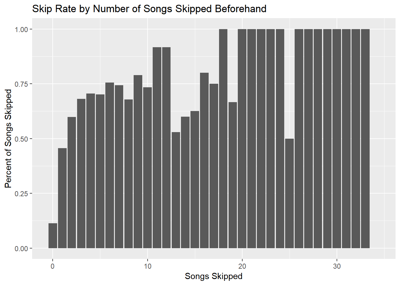 We can see that skipping two or three songs before the current song greatly increases the likelihood that the current song will be skipped. This will be a good feature to use.
I’m also curious about what time of day I tend to skip songs.
track_data$end_time_formatted <- ymd_hm(track_data$endTime)
track_data$hour <- hour(track_data$end_time_formatted)
track_data$weekday <- wday(track_data$end_time_formatted)
track_data %>%
group_by(hour) %>%
summarise(percent_skipped = sum(skipped, na.rm=TRUE)/n()) %>%
ggplot(aes(x = hour)) +
geom_bar(aes(weight=percent_skipped))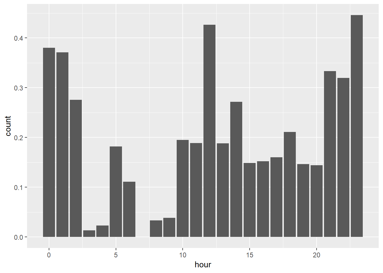
I see a spike after lunch and during the night, while early morning and early work hours appear below average.
We can also use the Spotify API to get features like “danceability” and “instrumentalness” from the song audio.
get_track_analysis_features <- function(track_id){

  query_response <- GET(paste0("https://api.spotify.com/v1/audio-features/",track_id),
                        add_headers(Authorization = auth_code)
  )
  #get the json response
  parsed_query_response <- tryCatch(content(query_response, "parsed"), error=function(e) NA)
  # print(parsed_query_response)
  as.data.frame(parsed_query_response)
}
Use a sample query to get the column names.
test_track_features <- get_track_analysis_features("0aNyZsNQZykSvoiwrjhBFB")
track_analysis_features_names <- names(test_track_features)
Query audio analysis features for every track ID we were able to find.
#create an empty dataframe with the right names
track_analysis_features <- data.frame(matrix(ncol = 18, nrow = 0))
colnames(track_analysis_features) <-  track_analysis_features_names

for (row in 1:nrow(track_data)) {
  track_id <- track_data[row,]$track_id

  #get track features
  current_track_analysis_features <- get_track_analysis_features(track_id)
  #create an NA dataframe on failure
  if(ncol(current_track_analysis_features) != 18){
    current_track_analysis_features <- data.frame(matrix(ncol = 18, nrow = 1))
    colnames(current_track_analysis_features) <- track_analysis_features_names
  }
  track_analysis_features <- rbind(track_analysis_features,
                                   current_track_analysis_features)
}str(track_analysis_features)## 'data.frame': 3654 obs. of 18 variables:
## $ danceability : num NA 0.358 0.666 0.377 0.534 0.713 0.785 NA 0.518 0.497 ...
## $ energy : num NA 0.232 0.432 0.00868 0.445 0.433 0.362 NA 0.585 0.523 ...
## $ key : int NA 6 6 0 7 9 9 NA 8 7 ...
## $ loudness : num NA -13.8 -8.79 -32.79 -9.62 ...
## $ mode : int NA 0 1 1 0 0 1 NA 1 1 ...
## $ speechiness : num NA 0.038 0.0323 0.0487 0.0351 0.0959 0.0611 NA 0.344 0.0322 ...
## $ acousticness : num NA 0.956 0.334 0.993 0.0483 0.0659 0.697 NA 0.347 0.881 ...
## $ instrumentalness: num NA 8.96e-01 2.89e-02 8.92e-01 7.25e-05 8.94e-01 3.34e-01 NA 9.08e-01 5.30e-01 ...
## $ liveness : num NA 0.106 0.11 0.0696 0.116 0.0992 0.0502 NA 0.111 0.212 ...
## $ valence : num NA 0.0742 0.297 0.0461 0.0828 0.468 0.513 NA 0.487 0.149 ...
## $ tempo : num NA 121.9 96 86.1 156 ...
## $ type : chr NA "audio_features" "audio_features" "audio_features" ...
## $ id : chr NA "0aNyZsNQZykSvoiwrjhBFB" "7JJinw17P46NEPXimuRkvt" "4GbJgSLRK5XUkSJmDoeTz5" ...
## $ uri : chr NA "spotify:track:0aNyZsNQZykSvoiwrjhBFB" "spotify:track:7JJinw17P46NEPXimuRkvt" "spotify:track:4GbJgSLRK5XUkSJmDoeTz5" ...
## $ track_href : chr NA "https://api.spotify.com/v1/tracks/0aNyZsNQZykSvoiwrjhBFB" "https://api.spotify.com/v1/tracks/7JJinw17P46NEPXimuRkvt" "https://api.spotify.com/v1/tracks/4GbJgSLRK5XUkSJmDoeTz5" ...
## $ analysis_url : chr NA "https://api.spotify.com/v1/audio-analysis/0aNyZsNQZykSvoiwrjhBFB" "https://api.spotify.com/v1/audio-analysis/7JJinw17P46NEPXimuRkvt" "https://api.spotify.com/v1/audio-analysis/4GbJgSLRK5XUkSJmDoeTz5" ...
## $ duration_ms : int NA 229853 270476 342857 188664 182784 148156 NA 225973 226977 ...
## $ time_signature : int NA 4 4 3 4 3 4 NA 5 3 ...Combine track data and analysis features for the full set of features.
track_data_features_full <- cbind(track_data, track_analysis_features)str(track_data_features_full)## 'data.frame': 3654 obs. of 32 variables:
## $ endTime : chr "2018-11-19 17:45" "2018-11-19 17:48" "2018-11-19 17:52" "2018-11-19 17:58" ...
## $ artistName : chr "Maribou State" "Will Stratton" "Elder Island" "Shanic" ...
## $ trackName : chr "Beginner's Luck" "Hemet Pine Singer" "Welcome State" "It All Changed So Fast" ...
## $ msPlayed : int 268027 191735 270476 342857 188664 182783 148155 163813 225973 226976 ...
## $ track_id : chr NA "0aNyZsNQZykSvoiwrjhBFB" "7JJinw17P46NEPXimuRkvt" "4GbJgSLRK5XUkSJmDoeTz5" ...
## $ track_album_id : chr NA "7Fitd8mCCAxXbbE5d6jfoE" "7MRtAyLQCuhaWSNtkb7Jqa" "4IWnOazPfcc5bXTHjZGwtO" ...
## $ track_artist_id : chr NA "0LyfQWJT6nXafLPZqxe9Of" "3EnbnmqrrvApHJs6FMvYik" "4iwYvUGOkgKYbCF0rcmJay" ...
## $ track_duration : int NA 229853 270476 342857 188664 182783 148155 NA 225973 226976 ...
## $ track_popularity : int NA 61 59 33 52 33 50 NA 55 31 ...
## $ skipped : logi NA TRUE FALSE FALSE FALSE FALSE ...
## $ skip_streak : num 0 0 1 0 0 0 0 0 0 0 ...
## $ end_time_formatted: POSIXct, format: "2018-11-19 17:45:00" "2018-11-19 17:48:00" ...
## $ hour : int 17 17 17 17 18 18 18 18 18 18 ...
## $ weekday : num 2 2 2 2 2 2 2 2 2 2 ...
## $ danceability : num NA 0.358 0.666 0.377 0.534 0.713 0.785 NA 0.518 0.497 ...
## $ energy : num NA 0.232 0.432 0.00868 0.445 0.433 0.362 NA 0.585 0.523 ...
## $ key : int NA 6 6 0 7 9 9 NA 8 7 ...
## $ loudness : num NA -13.8 -8.79 -32.79 -9.62 ...
## $ mode : int NA 0 1 1 0 0 1 NA 1 1 ...
## $ speechiness : num NA 0.038 0.0323 0.0487 0.0351 0.0959 0.0611 NA 0.344 0.0322 ...
## $ acousticness : num NA 0.956 0.334 0.993 0.0483 0.0659 0.697 NA 0.347 0.881 ...
## $ instrumentalness : num NA 8.96e-01 2.89e-02 8.92e-01 7.25e-05 8.94e-01 3.34e-01 NA 9.08e-01 5.30e-01 ...
## $ liveness : num NA 0.106 0.11 0.0696 0.116 0.0992 0.0502 NA 0.111 0.212 ...
## $ valence : num NA 0.0742 0.297 0.0461 0.0828 0.468 0.513 NA 0.487 0.149 ...
## $ tempo : num NA 121.9 96 86.1 156 ...
## $ type : chr NA "audio_features" "audio_features" "audio_features" ...
## $ id : chr NA "0aNyZsNQZykSvoiwrjhBFB" "7JJinw17P46NEPXimuRkvt" "4GbJgSLRK5XUkSJmDoeTz5" ...
## $ uri : chr NA "spotify:track:0aNyZsNQZykSvoiwrjhBFB" "spotify:track:7JJinw17P46NEPXimuRkvt" "spotify:track:4GbJgSLRK5XUkSJmDoeTz5" ...
## $ track_href : chr NA "https://api.spotify.com/v1/tracks/0aNyZsNQZykSvoiwrjhBFB" "https://api.spotify.com/v1/tracks/7JJinw17P46NEPXimuRkvt" "https://api.spotify.com/v1/tracks/4GbJgSLRK5XUkSJmDoeTz5" ...
## $ analysis_url : chr NA "https://api.spotify.com/v1/audio-analysis/0aNyZsNQZykSvoiwrjhBFB" "https://api.spotify.com/v1/audio-analysis/7JJinw17P46NEPXimuRkvt" "https://api.spotify.com/v1/audio-analysis/4GbJgSLRK5XUkSJmDoeTz5" ...
## $ duration_ms : int NA 229853 270476 342857 188664 182784 148156 NA 225973 226977 ...
## $ time_signature : int NA 4 4 3 4 3 4 NA 5 3 ...With that, I think we have enough features. We don’t need all the columns to train the model so we can select only the columns we need.
track_data_features <- track_data_features_full %>%
  select(
    skipped,
    skip_streak,
    hour,
    weekday,
    track_popularity,
    danceability,
    energy,
    key,
    loudness,
    mode,
    speechiness,
    acousticness,
    instrumentalness,
    liveness,
    valence,
    tempo
  ) %>%
  na.omit()
#convert to factor for random forest classification
track_data_features$skipped <- as.factor(track_data_features$skipped)
Random Forest
It’s time to create the prediction model. First, we have to separate the data into training testing sets.
set.seed(100)
train <- sample(nrow(track_data_features), 0.7*nrow(track_data_features), replace = FALSE)
train_set <- track_data_features[train,]
valid_set <- track_data_features[-train,]
summary(train_set)
## skipped skip_streak hour weekday
## FALSE:1407 Min. : 0.000 Min. : 0.0 Min. :1.000
## TRUE : 520 1st Qu.: 0.000 1st Qu.:11.0 1st Qu.:2.000
## Median : 0.000 Median :16.0 Median :4.000
## Mean : 1.162 Mean :13.9 Mean :3.919
## 3rd Qu.: 1.000 3rd Qu.:20.0 3rd Qu.:6.000
## Max. :33.000 Max. :23.0 Max. :7.000
## track_popularity danceability energy key
## Min. : 0.00 Min. :0.0000 Min. :0.000175 Min. : 0.000
## 1st Qu.: 46.00 1st Qu.:0.3260 1st Qu.:0.215500 1st Qu.: 1.000
## Median : 55.00 Median :0.4900 Median :0.422000 Median : 4.000
## Mean : 53.48 Mean :0.4795 Mean :0.440038 Mean : 4.166
## 3rd Qu.: 59.00 3rd Qu.:0.6600 3rd Qu.:0.659000 3rd Qu.: 7.000
## Max. :100.00 Max. :0.9430 Max. :1.000000 Max. :11.000
## loudness mode speechiness acousticness
## Min. :-46.448 Min. :0.0000 Min. :0.00000 Min. :0.0000
## 1st Qu.:-21.152 1st Qu.:0.0000 1st Qu.:0.03600 1st Qu.:0.1190
## Median :-12.925 Median :1.0000 Median :0.04460 Median :0.3330
## Mean :-16.127 Mean :0.6772 Mean :0.09325 Mean :0.4278
## 3rd Qu.: -8.860 3rd Qu.:1.0000 3rd Qu.:0.08505 3rd Qu.:0.7615
## Max. : -1.584 Max. :1.0000 Max. :0.72200 Max. :0.9960
## instrumentalness liveness valence tempo
## Min. :0.00000 Min. :0.02190 Min. :0.00000 Min. : 0.00
## 1st Qu.:0.00524 1st Qu.:0.09855 1st Qu.:0.07105 1st Qu.: 84.66
## Median :0.59700 Median :0.13500 Median :0.24400 Median :112.22
## Mean :0.50442 Mean :0.19532 Mean :0.32452 Mean :111.26
## 3rd Qu.:0.89900 3rd Qu.:0.22050 3rd Qu.:0.52300 3rd Qu.:130.01
## Max. :1.00000 Max. :0.98300 Max. :0.98000 Max. :209.77summary(valid_set)## skipped skip_streak hour weekday
## FALSE:609 Min. : 0.000 Min. : 0.00 Min. :1.000
## TRUE :218 1st Qu.: 0.000 1st Qu.:12.00 1st Qu.:3.000
## Median : 0.000 Median :16.00 Median :4.000
## Mean : 1.225 Mean :14.49 Mean :4.144
## 3rd Qu.: 1.000 3rd Qu.:20.00 3rd Qu.:6.000
## Max. :34.000 Max. :23.00 Max. :7.000
## track_popularity danceability energy key
## Min. : 4.00 Min. :0.0536 Min. :0.000224 Min. : 0.000
## 1st Qu.:46.50 1st Qu.:0.3650 1st Qu.:0.218000 1st Qu.: 1.000
## Median :55.00 Median :0.4900 Median :0.412000 Median : 3.000
## Mean :53.03 Mean :0.4839 Mean :0.446852 Mean : 4.053
## 3rd Qu.:59.00 3rd Qu.:0.6470 3rd Qu.:0.681500 3rd Qu.: 7.000
## Max. :96.00 Max. :0.9420 Max. :1.000000 Max. :11.000
## loudness mode speechiness acousticness
## Min. :-46.448 Min. :0.0000 Min. :0.02240 Min. :0.0000034
## 1st Qu.:-21.152 1st Qu.:0.0000 1st Qu.:0.03715 1st Qu.:0.1190000
## Median :-12.778 Median :1.0000 Median :0.04460 Median :0.3400000
## Mean :-15.977 Mean :0.6759 Mean :0.09703 Mean :0.4222262
## 3rd Qu.: -8.320 3rd Qu.:1.0000 3rd Qu.:0.09070 3rd Qu.:0.7795000
## Max. : -2.749 Max. :1.0000 Max. :0.72200 Max. :0.9960000
## instrumentalness liveness valence tempo
## Min. :0.000000 Min. :0.0244 Min. :0.00001 Min. : 46.95
## 1st Qu.:0.003755 1st Qu.:0.0995 1st Qu.:0.08140 1st Qu.: 86.99
## Median :0.597000 Median :0.1330 Median :0.26800 Median :115.03
## Mean :0.495254 Mean :0.1897 Mean :0.32827 Mean :112.85
## 3rd Qu.:0.893000 3rd Qu.:0.2130 3rd Qu.:0.52650 3rd Qu.:132.87
## Max. :0.985000 Max. :0.9770 Max. :0.97000 Max. :209.77I’m just going to use the defaults for this model. However, there are plenty of methods to use grid search and loop through parameters you can use if you want to get better predictions.
model <- randomForest(skipped ~ ., data = train_set, importance = TRUE, type = classification)model##
## Call:
## randomForest(formula = skipped ~ ., data = train_set, importance = TRUE, type = classification)
## Type of random forest: classification
## Number of trees: 500
## No. of variables tried at each split: 3
##
## OOB estimate of error rate: 18.37%
## Confusion matrix:
## FALSE TRUE class.error
## FALSE 1261 146 0.1037669
## TRUE 208 312 0.4000000One main reason I chose Random Forest was so I could get a clear view of the importance of each feature. It looks like skip streak is the best indicator by far.
importance(model)## FALSE TRUE MeanDecreaseAccuracy
## skip_streak 64.133308 72.4336116 82.919092
## hour 14.188931 8.8973681 16.730238
## weekday 9.918859 1.9784049 9.806679
## track_popularity 16.959472 4.0607791 17.598914
## danceability 13.535021 -1.0126104 12.151877
## energy 12.781509 10.2480297 16.862217
## key 6.443682 0.5880843 6.408745
## loudness 14.199997 11.8339001 18.386072
## mode 1.588636 0.7190802 1.798527
## speechiness 7.508636 7.4175950 10.124761
## acousticness 7.819603 5.0608135 10.453423
## instrumentalness 11.583550 12.0180676 15.658565
## liveness 10.215735 -1.2243800 9.088325
## valence 15.288138 -2.3483400 14.334362
## tempo 7.533527 5.7996491 9.323382
## MeanDecreaseGini
## skip_streak 193.773820
## hour 43.547560
## weekday 27.618062
## track_popularity 40.195048
## danceability 40.712076
## energy 47.766131
## key 23.635846
## loudness 53.806499
## mode 5.357875
## speechiness 38.896387
## acousticness 39.428905
## instrumentalness 50.586842
## liveness 36.065278
## valence 39.418151
## tempo 38.867707Overall, the prediction is pretty good.
predictions <- predict(model, newdata = valid_set)
table(predictions, valid_set$skipped)
##
## predictions FALSE TRUE
## FALSE 531 84
## TRUE 78 134There are a lot more features for tracks that Spotify exposes. Adding in more of these features could improve the performance of our predictions. It might also be interesting to do regression instead of classification and predict exactly how long you will listen to a song. There are a lot of interesting projects you can try with Spotify data, and I hope this tutorial helps get you started on your own.