Introduction

I have been curious about how I spend my time online and decided to investigate what activities I tend to do together in a single session. Association Rules allows us to discover the associations between these activities.

Association Rules

Association Rules is an algorithm to find patterns in events that tend to occur together. One common example is where a supermarket used this algorithm to discover that people who buy diapers also tend to buy beer, later reasoning that there are a lot of new dads shopping. With this information you could decide to put diapers and beer close together to simplify the shopping experience. Or you could place diapers at the other end of the store to make new dads walk by temptations of grills, sandals, and football merchandise.

Definition: Frequent Itemsets

An itemset is a collection one or more items. First, start with a dataframe of itemsets

Transaction ID	Items
1	Bread, Milk
2	Bread,Diaper,Beer,Eggs
3	Milk,Diaper,Beer,Coke
4	Bread,Milk,Diaper,Beer
5	Bread,Milk,Diaper,Coke

The support count is how many times an itemset occurred. e.g The support count of {Milk,Bread,Diaper} = 2

The support is the fraction of all transactions that contain an itemset. e.g. The support of {Milk,Bread,Diaper} = 2/5

The first parameter we need to manually set in Association Rules is a minimum support. A frequent itemset is any itemset that has a support greater than or equal to the minimum support. Within the Association Rules algorithm we will filter to only use frequent itemsets to save computation time.

Definition: Association Rule

An Association Rule takes the form of X -> Y.

For example, {Milk,Diaper} -> {Beer} means that a transaction where someone bought milk and diapers implies that they also bought beer.

Support

Support has the same meaning as with an itemset, but the itemset you are counting is both sides of the implication

e.g. support for {Milk,Diaper} -> {Beer} is support_count({Milk,Diaper,Beer})/count(transactions) = 2/5

The second parameter is a confidence threshold.

Confidence

Confidence is a measure of how often items in Y also appear in transactions that contain X.

c = support_count({Milk,Diaper,Beer})/support_count(Milk,Diaper) = 2/3

A higher confidence means that the outcome has a greater frequency to occur in the set rather than outside of it. Note that you can have the same itemset, but depending on how the rule is formed, confidence may change. For example

{Milk} -> {Diaper,Beer} has a support of 0.4 and a confidence of 0.5. {Milk,Beer} -> {Diaper} has a support of 0.4, but a confidence of 1.0

So if milk is bought there is a 50% chance of also buying diapers and beer. However, if milk and beer are bought, then there is a 100% chance of purchasing diapers.

The last main metric often observed in association rules is lift.

Lift

Confidence tells you if the right side is more likely to occur given the left side. However, that isn’t always enough. Consider the following example of drinkers of coffee and tea. 100 people were asked if they drink coffee and tea. To relate to Association Rules you can think of this as 100 restaurant orders where people had tea or coffee.

	Coffee	Not(Coffee)
Tea	15	5	20
Not(Tea)	75	5	80
	90	10	100

The confidence of someone drinking coffee given that they drink tea is 15/20 or 75%, pretty high. That means that we are confident that someone drinking tea also drinks coffee. Giving us the rule {Tea} -> {Coffee}. However, the probability that someone drinks coffee disregarding tea is 90/100 or 90%. Therefore, if someone drinks tea they are less likely to drink coffee than someone who doesn’t drink tea. With this knowledge {Tea} -> {Coffee} doesn’t make as much sense as {} -> {Coffee}.

{} denotes empty set, indicating that every transaction implies the right hand itemset

Lift fixes this by accounting for that probability that someone drinks coffee.

In this example lift = 0.75/0.9 = 0.83. Since it is less than one, drinking coffee is negatively associated with drinking tea.

Using lift we can filter for rules where the resulting item is more likely to occur given the input itemset.

Format the Data

The data I’ll be using is from RescueTime. I went through how to retrieve this data in my previous post How to Download and Analyze Your RescueTime Data in R. I’m only going look at categories of websites. However, you can use the same method to look at specific websites. You can even try this with Google History from Takeout, but it would take more formatting to categorize websites from raw URLs or titles.

library(lubridate)
rescue.documents <- read.csv("../data/rescuetime-activity-history.csv", stringsAsFactors = FALSE, header=FALSE)
names(rescue.documents) <-  c("time", "activity","title", "category","domain", "duration")
rescue.documents$time <- mdy_hm(rescue.documents$time)
str(rescue.documents)

## 'data.frame':    241 obs. of  6 variables:
##  $ time    : POSIXct, format: "2018-09-14 01:00:00" "2018-09-14 01:00:00" ...
##  $ activity: chr  "rstudio" "newtab" "docs.google.com/#document" "docs.google.com/#document" ...
##  $ title   : chr  "C:/Users/Will/Desktop/Personal Projects/PersonalSite - master - RStudio" "New Tab - Google Chrome" "Google Docs - Google Chrome" "Untitled document - Google Docs - Google Chrome" ...
##  $ category: chr  "Software Development" "Utilities" "Design & Composition" "Design & Composition" ...
##  $ domain  : chr  "Data Modeling & Analysis" "Browsers" "Writing" "Writing" ...
##  $ duration: int  306 18 11 10 3 3327 114 43 26 15 ...

As always, there is a bit of cleaning to do before we can run the algorithm.

Create Sessions

Start out by including tidyverse.

library(tidyverse)

In order for Association Rules to work, we need to define what counts as a transaction or web session. Whether you get web history from Google or RescueTime, there isn’t a strict definition of what counts as a session. I’m defining a session as continuous web usage with breaks no longer than 60 minutes.

The following function creates sessions from a timestamp column.

make.sessions <- function(time.vec, time.sep = 30, time.unit = "mins"){
  #create a vector of next times
  lag.vec <- lag(time.vec)
  #find the difference in time between web activity
  difftime.vec <-  difftime(time.vec,lag.vec, units=time.unit)
  #stop if any difference is negative
  stopifnot(difftime.vec[!is.na(difftime.vec)] >= 0)
  #set all points where there is a new session to 1 and 0 otherwise
  new.sessions <- as.numeric(difftime.vec > as.difftime(time.sep, units = time.unit))
  new.sessions[is.na(new.sessions)] <- 0
  #use addition to create indexes
  sessions <- cumsum(new.sessions)
}

Run the function on RescueTime data and view the results. Make sure your data is sorted by time before using this function.

rescue.documents <- rescue.documents %>% arrange(time)
rescue.documents$session.id <-  make.sessions(rescue.documents$time, time.sep = session.break.time)

Format Session Data for Rransactions

Within a single session there are likely duplicate websites and categories. Since Association Rules is based on set manipulation, we don’t need those duplicates and can simplify our dataframe by removing them.

rescue.sessions.unique.categories <-  rescue.documents %>% group_by(category, session.id) %>% dplyr::summarise(count = n())

Lets look at the dataframe we’ll coerce into a transaction.

summary(rescue.sessions.unique.categories)

##    category           session.id       count       
##  Length:16878       Min.   :   0   Min.   :  1.00  
##  Class :character   1st Qu.: 605   1st Qu.:  2.00  
##  Mode  :character   Median :1430   Median :  5.00  
##                     Mean   :1355   Mean   : 12.83  
##                     3rd Qu.:2041   3rd Qu.: 15.00  
##                     Max.   :2650   Max.   :895.00

The arules library uses a specific transaction data format. To convert the dataframe into a transaction first create a vector of comma-separated items, then use the as function to coerce the vector into a transactions object.

library(arules)
categories.in.session <- aggregate(category ~ session.id, data = rescue.sessions.unique.categories, c)
category.transactions <- as(categories.in.session$category, "transactions")

Run Association Rules

category.rules <- apriori(category.transactions, parameter = list(supp=0.1, maxlen=3))

## Apriori
## 
## Parameter specification:
##  confidence minval smax arem  aval originalSupport maxtime support minlen
##         0.8    0.1    1 none FALSE            TRUE       5     0.1      1
##  maxlen target   ext
##       3  rules FALSE
## 
## Algorithmic control:
##  filter tree heap memopt load sort verbose
##     0.1 TRUE TRUE  FALSE TRUE    2    TRUE
## 
## Absolute minimum support count: 265 
## 
## set item appearances ...[0 item(s)] done [0.00s].
## set transactions ...[11 item(s), 2651 transaction(s)] done [0.00s].
## sorting and recoding items ... [11 item(s)] done [0.00s].
## creating transaction tree ... done [0.00s].
## checking subsets of size 1 2 3 done [0.00s].
## writing ... [296 rule(s)] done [0.00s].
## creating S4 object  ... done [0.00s].

You can look through rules with the inspect function.

inspect(head(sort(category.rules, by="lift"), n=10))

##      lhs                             rhs                      support confidence     lift count
## [1]  {Business,                                                                                
##       Design & Composition}       => {Software Development} 0.2097322  0.8273810 2.206627   556
## [2]  {Communication & Scheduling,                                                              
##       Design & Composition}       => {Software Development} 0.2304791  0.8028909 2.141312   611
## [3]  {Design & Composition,                                                                    
##       Social Networking}          => {Software Development} 0.1942663  0.8009331 2.136090   515
## [4]  {Design & Composition,                                                                    
##       Software Development}       => {Business}             0.2097322  0.8348348 1.990240   556
## [5]  {Social Networking,                                                                       
##       Software Development}       => {Business}             0.2195398  0.8151261 1.943255   582
## [6]  {Communication & Scheduling,                                                              
##       Software Development}       => {Business}             0.2542437  0.8120482 1.935917   674
## [7]  {Communication & Scheduling,                                                              
##       Design & Composition}       => {Business}             0.2297246  0.8002628 1.907821   609
## [8]  {Shopping,                                                                                
##       Software Development}       => {Uncategorized}        0.1086382  0.9664430 1.603279   288
## [9]  {Design & Composition,                                                                    
##       Shopping}                   => {Uncategorized}        0.1029800  0.9479167 1.572545   273
## [10] {Business,                                                                                
##       Shopping}                   => {Uncategorized}        0.1256130  0.9433428 1.564957   333

You can also coerce them into a dataframe if you prefer.

df_rules <- as(sort(category.rules, by="lift"),"data.frame")
head(df_rules)

##                                                                           rules
## 103                   {Business,Design & Composition} => {Software Development}
## 108 {Communication & Scheduling,Design & Composition} => {Software Development}
## 104          {Design & Composition,Social Networking} => {Software Development}
## 102                   {Design & Composition,Software Development} => {Business}
## 155                      {Social Networking,Software Development} => {Business}
## 159             {Communication & Scheduling,Software Development} => {Business}
##       support confidence     lift count
## 103 0.2097322  0.8273810 2.206627   556
## 108 0.2304791  0.8028909 2.141312   611
## 104 0.1942663  0.8009331 2.136090   515
## 102 0.2097322  0.8348348 1.990240   556
## 155 0.2195398  0.8151261 1.943255   582
## 159 0.2542437  0.8120482 1.935917   674

Visualize

You can also visualize Association Rules with some arulesViz. When I use Association Rules, it’s generally very exploratory. This package makes exploring rules very easy and even offers interactive modes.

library(arulesViz)

The default plot helps identify the distribution of rules over confidence, support, and lift.

plot(category.rules)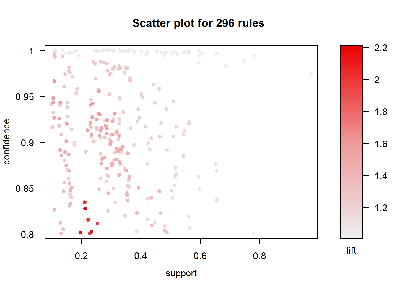

You can also use the interactive plot to view the actual rules behind each data point.

plot(category.rules, engine="htmlwidget")

## Warning: package 'bindrcpp' was built under R version 3.4.4

The paracoord plot helps view how items place into rules.

plot(category.rules, method="paracoord",  control=list(alpha=.5, reorder=TRUE))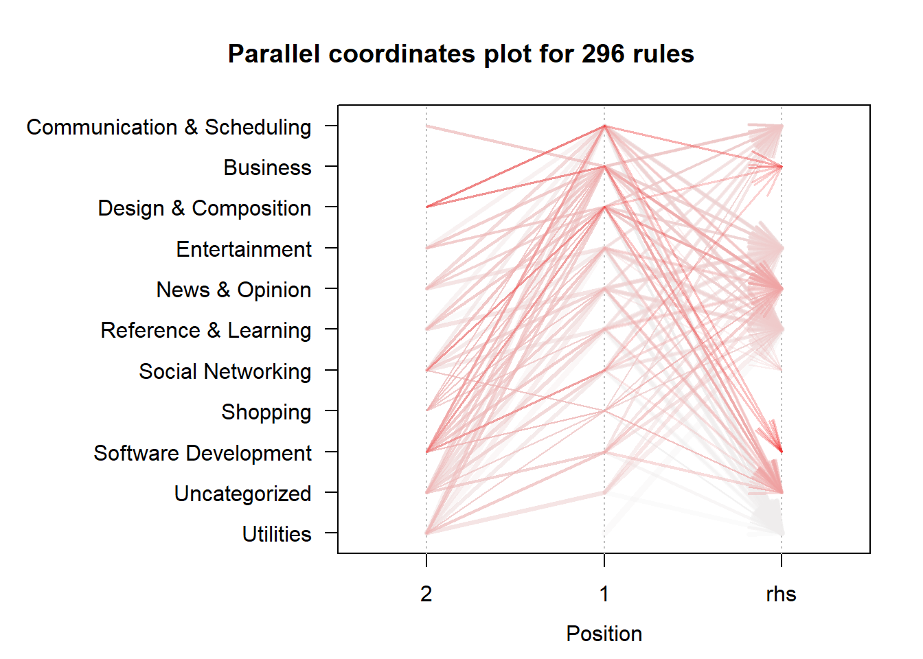

My favorite is to simply view all the rules in an interactive table. This allows you to sort and search for rules dynamically.

inspectDT(category.rules)

This interactive mode is especially useful with a large number of rules, which is hard to visualize. I recommend trying it if you decide to do rules on websites visited rather than categories of websites.

There we have it. You can run Association Rules any time it makes sense to think in terms of transactions where multiple things may be done together. Next time I’ll have to see what arises when I switch to sequential pattern analysis.

Association Rules in Web History